ENG/ESP
ENG
COMPARISON OF SEVERAL GLIDER FEATURES
USING THE SOFTWARE XFLR5
Chapter 1


We start in this article a series that tries to apply to close examples to model gliders the powerful capacity of analysis of the tool XFLR5, I have not found much written in Spanish. It is not intended to be a manual or a textbook but tries to help to use XFLR5 and to better understand the behavior of our models. These articles are written with humility within what my limited ability has been able to synthesize and explain. I beg the reader to send me their doubts and inaccuracy notices freely to the mail below.
XFLR5 is a tool developed BY Andre Deperrois and others, it has been improved since 2003 actively. XFLR5 is distributed as free software under GNU public license (http://www.xflr5.com). The root of XFLR5 is the SW XFOIL.
XFOIL is a development of Mark Drela y Harold Youngren (http://web.mit.edu/drela/Public/web/xfoil) in the middle 80´s of former century in Massachusetts Institute of Technology. The biggest contribution of XFOIL to the scientific community in the field of numeric analysis of fluid mechanics is the coupling of the solution for solving the boundary layer equations with the solution of the external flows around an airfoil.
The publication of XFOIL as free GNU SW was a global shock at academic level both for the revolutionary of the applied approach and for the generosity of the authors to bring within the reach of the big audience, the institutions and the industry of such a powerful and simple tool. Think of this was the moment of the main frames and the early stages of personal computers and workstations.
XFOIL is written in Fortran 77 and still it is so nowadays and still used in many professional applications. By 97-98 Drela published that XFOIL would not be improved anymore (though still today there are regular updates, last one December 2013).
Using XFOIL one can predict, with outstanding accuracy, a given profile’s behavior at different angles of attack and speeds (Reynolds number), that is to say the polar of such profile. Like a virtual wind tunnel. (To learn more on wind tunnels and polar evaluation at low Reynolds numbers see http://m-selig.ae.illinois.edu/ads.html , this site is sponsored by Illinois University and Prof. Michael Selig).
We can also use XFOIL for designing a profile which can feature a given pressure distribution along its chord.
Since XFOIL is written in FORTRAN 77, it uses a command line interface (like that black screen that sometimes it has to be used in Windows computers and does not usually preclude good things…) despite is has been proven that this is the most productive approach for interfacing sw it does need a lot of training and some programming skills.
Mr. Deperrois challenge has been to translate the FORTRAN 77 code into a graphic environment like Windows and he and his team have recoded and validated extensively XFOIL into a C++ application where with little effort we can start getting analysis results from profiles.
But this is not the only thing XFLR5 brings. XFOIL perform analysis in 2 dimensions, like a wing with infinite span and every slice we cut has the same airflow and more.
We all know the wings of our airplanes do have a finite span and the flow around our airfoils is quite different in each section: it appears the perverse effect of 3 dimensional flows and the “induced” drag.
Well, a part of replicating all XFOIL characteristics XFLR wants to simulate the airflow around the entire model, the wing with its three dimensional flow, its interaction with the control surfaces and eventually the fuselage. Furthermore it is also able to predict the coefficients of stability of the apparatus around its three axes. The work is immense and it is not surprising that the evolution of XFLR5 is over the years … and what still remains.
On paper one might think that XFLR5 would allow designing a plane completely, and it is, but the author himself advises against its use in anything other than model aircraft, there are several mathematical and model assumptions, that have not been supported neither mathematical nor formally in an experimental way which should be taken with caution like, for instance, that the wing sections continue to behave as if they were two-dimensional … Anyway, the results of XFLR would have been desired by many certified airplanes for their design and, for what we are interested in, XFLR5 is a reference program and like all the applications: its results will never be able to improve the quality of the data fed to it.
Creating a Model: The Supra.
I have chosen this model for many reasons … The main one is that it is a very well documented design (http://www.charlesriverrc.org/articles/supra/supra.htm). Of course, as it could not be otherwise, it is a design by Professor Drela, which was published in 2004 and has also been a emotional shock in the construction of F3J gliders and has been replicated many times by many model aircraft and is commercially exploited.
The profiles.
Supra´s wing profiles are the AG40d AG41d AG42d Y AG43d from wing root to wing tip with a thickness from 8% to 6,5%, (we know this is for structural reasons).
These profiles are designed to have a hinge, 75% flap of its chord.
The information provided in the .dat files corresponds to the profile with a deflection of two degrees (-2) upwards.

AG40d-2f, profile as tabulated.
We all know that we normally have in a F5J glider three flight modes «cruise» another “thermal “and a «reflex» or high speed. This “reflex” mode is that of the above figure.
If we apply the flap hinge then we will have for the nominal deflection or 0 degrees:

And for a +3 degrees deflection the “thermal”:

The reader can draw now the following conclusions.
a) To do a good analysis we usually put many points where the fluid happens to have important things such as on the leading edge and here we see in the area of the hinge.
b) It is much easier and more precise to cut and fabricate the -02f section, the original one that is practically flat bottom than the two below (and it is a good thing we have drawn the horizontal reference line because otherwise it would be difficult to see the difference between the two first profiles). Difference so small? We will see that it is more than important.
c) The nominal profile ( the yellow, + 00f) is continuous in the extrados. You see that this flap position is the design position. Since the flow and its control by the area of the suction side is the most sensitive part for the correct functioning of a profile.
These reasons are very important when it comes to understanding why AG profiles are so popular in the world of model airplanes.
In summary for our model to analyze we have already defined the sections of its wings and the three representative geometries for its flight modes. These sections should be conveniently placed along the wingspan in the geometric definition of the wing.
Then we continue positioning the sections of the tail, Stabilizer: Profiles HT14 in the root and HT12 in the marginal and Rudder HT13 and HT12.
(And after several weeks of fights with the geometry of the fuselage ….)
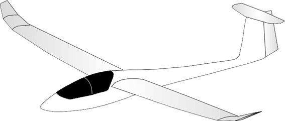
This will be the reference Supra, which draws XFLR5, for successive analyzes:

Copyright (C) 2017 Javier Hernández Rodero.
Permission is granted to copy, distribute and/or modify this document
under the terms of the GNU Free Documentation License, Version 1.3
or any later version published by the Free Software Foundation;
with no Invariant Sections, no Front-Cover Texts, and no Back-Cover Texts.
A copy of the license is included in the section entitled «GNU
Free Documentation License». http://www.gnu.org/licenses/fdl-1.3.html
Javier Hernández Rodero builds his own planes, with help from his friends and can be contacted in: japi (at) clubpetirrojo (punto) com
ESP
COMPARACION DE VARIAS CARACTERISTICAS DE PLANEADORES
USANDO EL PROGRAMA XFLR5
Iniciamos en este articulo una serie que intenta aplicar a ejemplos próximos de los modelo planeadores la potente capacidad de análisis de la Herramienta XFLR5, sobre la que no he encontrado mucho escrito en castellano. No pretende ser un manual ni tampoco un libro de texto pero sí ayudar a utilizar XFLR5 y a entender mejor el comportamiento de nuestros modelos. Estos artículos están escritos con humildad dentro de lo que mi limitada capacidad ha sido capaz de sintetizar y explicar. Ruego a lector me haga llegar sus dudas y avisos de incorrecciones con toda libertad al correo de más abajo.
La Herramienta XFLR5 Es un desarrollo de Andre Deperrois y otros, que desde 2003 se viene mejorando activamente. XFLR5 se distribuye como SW libre bajo licencia publica GNU (http://www.xflr5.com). La semilla de XFLR5 es el SW XFOIL .
XFOIL es un desarrollo de Mark Drela y Harold Youngren (http://web.mit.edu/drela/Public/web/xfoil) a mediados de los 80 del siglo XX en el Instituto Tecnológico de Massachusetts. La gran aportación de XFOIL a la comunidad científica en el campo de análisis numérico de la mecánica de fluidos es el acoplamiento de la resolución de la capa límite con la solución de la corriente exterior alrededor de un perfil.
La publicación de XFOIL como SW libre GNU fue una conmoción mundial a nivel académico tanto por lo revolucionario de la metodología aplicada como por la generosidad de los autores al poner al alcance del gran público, las instituciones y las empresas una herramienta tan potente y sencilla. Piénsese que era la época de los “mainframes” y los albores del ordenador personal.
XFOIL está escrito en Fortran 77 y todavía está hoy en día más o menos actualizado en multitud de aplicaciones profesionales. A partir del 97-98 Drela publicó que XFOIL no se mejoraría más (aunque todavía hay actualizaciones regulares, la última de Diciembre 2013).
Con XFOIL se puede predecir, con una precisión sorprendente, el comportamiento a diferentes ángulos de ataque y velocidad (número de Reynolds) de un perfil dado, o sea dibujar la polar de ese perfil. Como si de un túnel de viento virtual se tratara. (Para saber más de túneles de viento y evaluación de polares de perfiles a bajo número de Reynolds ver http://m-selig.ae.illinois.edu/ads.html , sitio auspiciado por la Universidad de Illinois y el Prof. Michael Selig).
También se puede usar XFOIL para diseñar un perfil que tenga una determinada distribución de presión a lo largo de su cuerda.
Como XFOIL está escrito en FORTRAN, su interface es a base de comandos de línea (sí, como esa pantalla negra que a veces hay que usar en los ordenadores Windows y que, por lo general, trae malos augurios…) que, aunque está demostrado que es la manera más eficaz de operar, necesita de un alto nivel de habilidades de programación y de entrenamiento en la aplicación.
El desafío del Mr. Deperrois ha sido transferir el código de FORTRAN 77 a un entorno gráfico tipo Windows y ha recodificado, y validado, XFOIL al lenguaje C++ en donde con poco esfuerzo se pueden empezar a obtener resultados de análisis de perfiles.
Pero allí no para la cosa. XFOIL hace análisis de perfiles en dos dimensiones, como si de un ala con ese perfil fuera infinitamente ancha y haciendo un corte por cualquier sección el aire a su alrededor se mueve siempre de la misma manera.
Todos sabemos que las alas las de nuestros modelos, y de todos los aviones, tienen una dimensión finita y el flujo alrededor de nuestros perfiles es muy diferente en cada sección: aparecen los perversos efectos de “resistencia inducida” y de “flujo tridimensional”.
Bien, pues aparte de replicar todas las características de XFOIL el programa XFLR quiere simular TODO el modelo, su ala con efectos tridimensionales y su interacción con las superficies estabilizadoras y, eventualmente el fuselaje. Además es capaz de predecir los coeficientes de estabilidad del aparato alrededor de sus tres ejes. El trabajo es inmenso y no es de extrañar que la evolución de XFLR5 sea a lo largo de años… y lo que queda.
Sobre el papel uno podría pensar que XFLR5 permitiría diseñar un avión completamente, y se podría, pero el mismo autor desaconseja su utilización en algo diferente de aeromodelos, existen ciertas simplificaciones matemáticas que se han hecho, que no han sido soportadas ni matemática ni formalmente de una manera experimental que deben ser tomadas con precaución como por ejemplo que las secciones del ala siguen comportándose como si fueran bidimensionales… De todas maneras los resultados de XFLR ya quisieran muchos aeroplanos certificados haber contado con ellos para su diseño y para lo que a nosotros nos interesa XFLR5 es un programa de referencia y como todas las aplicaciones informáticas: sus resultados nunca podrán mejorar la calidad de los datos de partida suministrados.
Creando un Modelo: El Supra, he elegido este modelo por muchas razones… La principal es que es un diseño que está muy bien documentado (http://www.charlesriverrc.org/articles/supra/supra.htm). Claro, como no podía ser de otra manera, es un diseño del Profesor Drela, que se publicó en 2004 y que también ha sido una conmoción en la construcción de veleros F3J y que ha sido replicado multitud de veces por muchos aeromodelistas y se explota comercialmente.
Los Perfiles.
Los perfiles del ala del Supra. Son los AG40d AG41d AG42d Y AG43d desde el encastre al borde marginal con un espesor relativo desde el 8% al 6,5%, (esto es por razones estructurales).
Estos perfiles están diseñados para tener una bisagra, flap al 75% de su cuerda
La información que se facilita en los archivos .dat es la que corresponde al perfil con una deflexión de dos grados (-2) hacia arriba.
Perfil AG40d-2f tal y como está tabulado.
Todos sabemos que normalmente se tienen en un velero de F5J tres modos de vuelo de “crucero” otro térmico y uno “réflex” o de alta velocidad. Este Modo réflex es el de la figura de más arriba.
Si aplicamos la bisagra del flap entonces tendremos para la deflexión nominal o sea 0 grados:
Y para la deflexión +3 grados o térmica:
El lector podrá sacar ya las siguientes conclusiones.
- a) para hacer un buen análisis normalmente se ponen muchos puntos en donde al fluido le pasan cosas importantes como por ejemplo en el borde de ataque y aquí vemos en la zona de la bisagra.
- b) Es muucho más fácil y preciso cortar y fabricar la sección -02f, la original que es prácticamente plana que las dos de más abajo ( y menos mal que hemos dibujado la línea de referencia horizontal porque si no sería complicado ver la diferencia entre ambos perfiles). Diferencia tan pequeña? Ya veremos que es más que importante.
- c) El perfil nominal (el amarillo, el +00f) es continuo en el extradós. Se ve que esa posición de flap es la de diseño. Ya que el flujo y su control por la zona de del extradós es la parte más sensible para el correcto funcionamiento de un perfil.
Estas razones son muy importantes a la hora de comprender por qué los perfiles AG son tan populares en el mundo de los aeromodelos.
En resumen para nuestro modelo a analizar ya tenemos definidas las secciones de sus alas y las tres geometrías representativas para sus modos de vuelo. Estas secciones deben ser colocadas convenientemente a lo largo de la envergadura en la definición geométrica del ala.
Luego continuamos posicionando las secciones de la cola, Estabilizador: Perfiles HT14 en la raíz y HT12 en el marginal y Timón HT13 y HT12.
(Y después de varias semanas de peleas con la geometría del fuselaje….)
Este será el Supra de referencia para los análisis sucesivos, que dibuja XFLR5:
Copyright (C) 2017 Javier Hernández Rodero.
Permission is granted to copy, distribute and/or modify this document
under the terms of the GNU Free Documentation License, Version 1.3
or any later version published by the Free Software Foundation;
with no Invariant Sections, no Front-Cover Texts, and no Back-Cover Texts.
A copy of the license is included in the section entitled «GNU
Free Documentation License». http://www.gnu.org/licenses/fdl-1.3.html
Javier Hernández Rodero se construye sus propios modelos, con ayuda de sus amigos y puede ser contactado en japi (at) clubpetirrojo (punto) com